In the previous blog post, we discussed how reinforcement learning can be interpreted as sampling from an energy-based distribution:
\[p(x)\propto p_{\mathrm{ref}}(x)\exp\left(-\frac{g(x)}{\beta}\right),\]where $g(x)$ is the objective to minimize (e.g., a cost or negative reward), $p_{\mathrm{ref}}(x)$ is a reference distribution, and $\beta$ controls the strength of regularization toward this reference.
In this post, we explore unsupervised training of diffusion models. Unlike models that generate samples in a single step, diffusion models introduce a sequence of intermediate latent states that progressively transform noise into data. We will examine this process from three complementary perspectives, each providing a different way to understand and optimize diffusion models without relying on training samples from the target distribution.
Before proceeding, let us clarify the notation. Discrete-time diffusion models and continuous-time formulations often adopt opposite time conventions, as illustrated below.
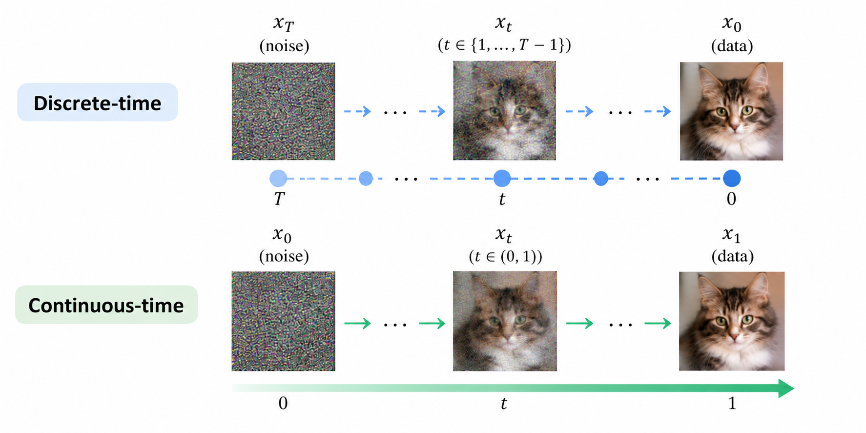
We will use the discrete-time convention in the first two sections and the continuous-time convention in the final section.
One subtlety is that, since the reference distribution $p_{\mathrm{ref}}(x)$ is generally intractable for diffusion models, we instead define the reference distribution over the entire generation trajectory. For a discrete-time process, this gives
\[\boxed{ \min_p \mathbb{E}_p[g(x_0)] + \beta D_{\mathrm{KL}}(p(x_{0:T})\|p_{\mathrm{ref}}(x_{0:T})) \quad \Rightarrow\quad p(x_{0:T}) \propto p_{\mathrm{ref}}(x_{0:T}) \exp\left(-\frac{g(x_0)}{\beta}\right). }\]Perspective 1: Langevin Dynamics
I personally find this the most intuitive perspective for understanding diffusion models.
One defining feature of diffusion models is their iterative generation process, in contrast to models such as VAEs and GANs. However, iterative sampling is not unique to diffusion models. As we discussed in the previous post, Markov Chain Monte Carlo (MCMC) also generates samples through a sequence of transitions.
The key distinction is:
- MCMC typically targets the same distribution throughout the sampling process.
- Diffusion models progressively move through different distributions, from noise toward the target distribution.
In this sense, diffusion models can be understood from the perspective of annealed MCMC, which also motivates Noise Conditional Score Networks (NCSN).
Recall that MCMC can be intuitively viewed as a stochastic hill-climbing process: we tend to move toward regions of higher probability while occasionally accepting moves toward lower-probability regions to maintain exploration.
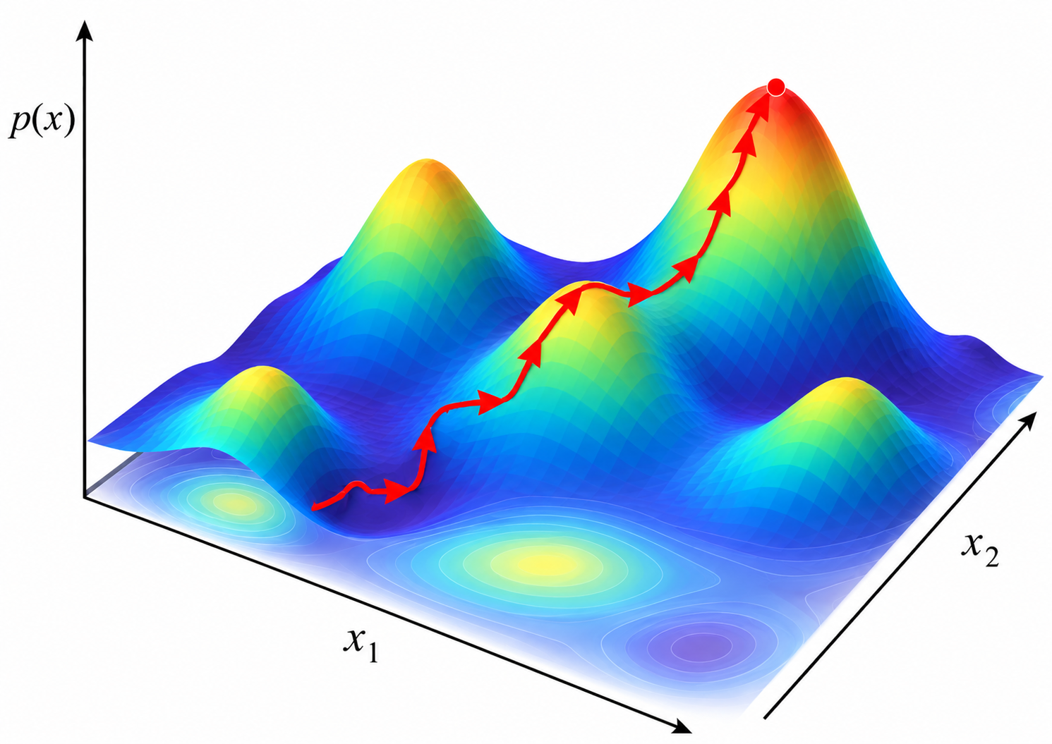
For example, in the Metropolis–Hastings algorithm, we first propose a new state:
\[x' \sim p_{\theta}(x'\mid x).\]We then decide whether to accept this proposal according to
\[A(x',x) = \min\left( 1, \frac{ p(x')p_{\theta}(x\mid x') }{ p(x)p_{\theta}(x'\mid x) } \right).\]For a symmetric proposal distribution, this simplifies to a particularly intuitive rule:
- If $p(x')\geq p(x)$, we always accept the new state.
- Otherwise, we accept it with probability $p(x')/p(x)$, allowing occasional moves toward less probable states.
The efficiency of MCMC depends heavily on the proposal distribution. A good proposal explores high-probability regions efficiently, whereas a poor proposal may waste many steps on rejected moves. This naturally raises a question:
Can we directly propose moves toward higher-probability regions?
Locally, the direction of steepest increase in $\log p(x)$ is given by its gradient $\nabla_x\log p(x)$, known as the score.
Using the score, we can construct a gradient-guided stochastic sampling process, known as Langevin dynamics:
\[x'=x+ \frac{\sigma^2}{2}\nabla_x \log p(x) + \sigma\,\xi, \qquad \xi\sim\mathcal N(0,I).\]The update has two components:
- Gradient ascent: $\frac{\sigma^2}{2}\nabla_x\log p(x)$ pushes the sample toward higher-probability regions.
- Random exploration: $\sigma\,\xi$ introduces stochasticity, allowing the process to explore the distribution rather than simply converge to a local mode.
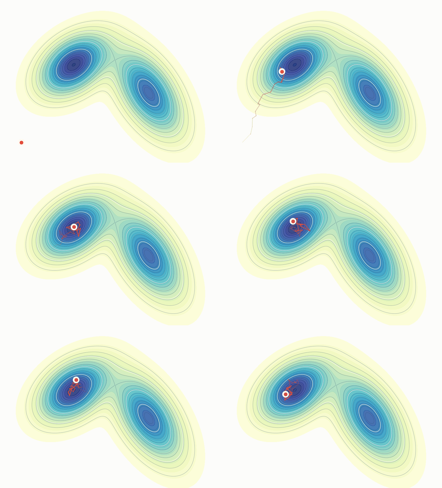
Unlike ordinary gradient ascent, which seeks a mode of the distribution, Langevin dynamics combines gradient information with noise to sample from the target distribution (up to discretization error for finite step sizes).
The remaining challenge is how to obtain the score $\nabla_x\log p(x)$ when the target density is unknown. This leads to an established family of methods known as score matching.
Since traditional score matching is not directly related to the unsupervised training methods we focus on here, I have included an optional explanation below, starting from the intuition behind density estimation and ending with the modern diffusion model objective.
Optional: how is the score actually estimated? (KDE, multi-noise-level training, and annealed Langevin dynamics)
Score matching aims to learn a function $s_{\theta}(x)$ that approximates the score of the data distribution:
\[\min_{\theta} \mathbb{E}_{p(x)}[\Vert s_{\theta}(x)-\nabla \log p(x)\Vert^2].\]The challenge is that we only observe samples $x\sim p(x)$ without knowing the density $p(x)$ itself, let alone its gradient $\nabla\log p(x)$. How can we learn something we cannot directly evaluate?
Let us first forget about the mathematical formulations and consider a simple example. Imagine a unit square containing a collection of observed samples. How would you estimate the probability density $p(x)$ at an arbitrary point?
One simple approach is to draw a small box around that point and count how many samples fall inside it. Dividing the count by the number of samples and the box area gives an estimate of the density. This is known as the Parzen window method.
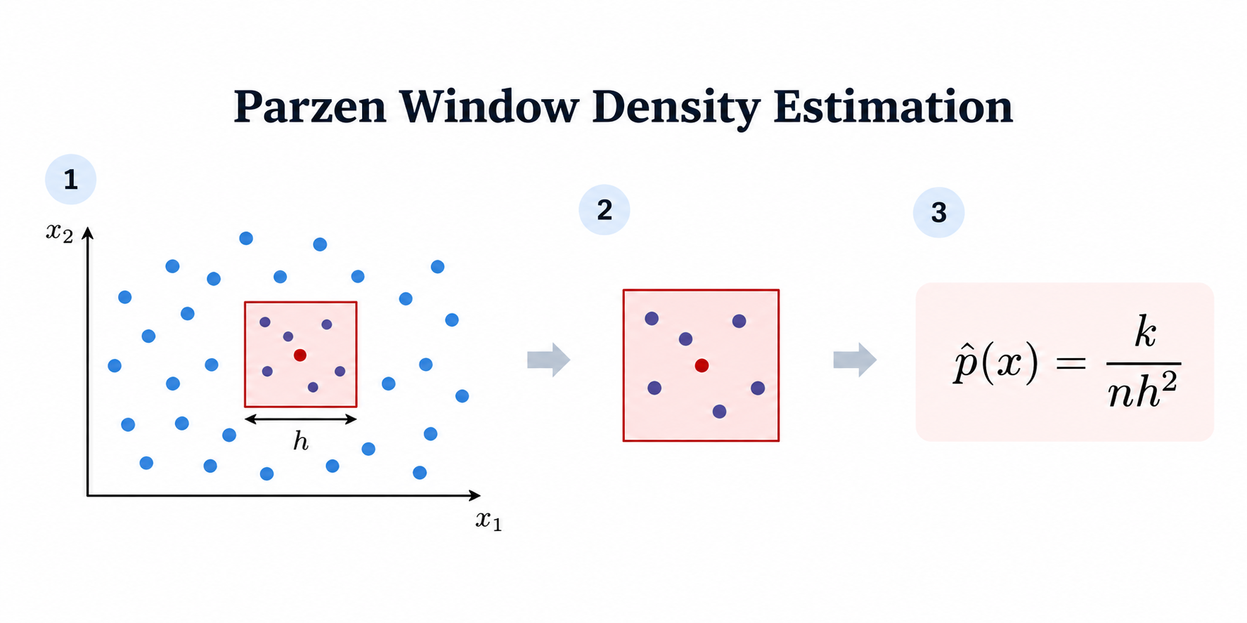
The Parzen window method uses a hard boundary: samples inside the window contribute equally, while samples outside contribute nothing.
A smoother alternative is to assign each sample a weight based on its distance from the target point, using a kernel function. This is known as kernel density estimation (KDE).
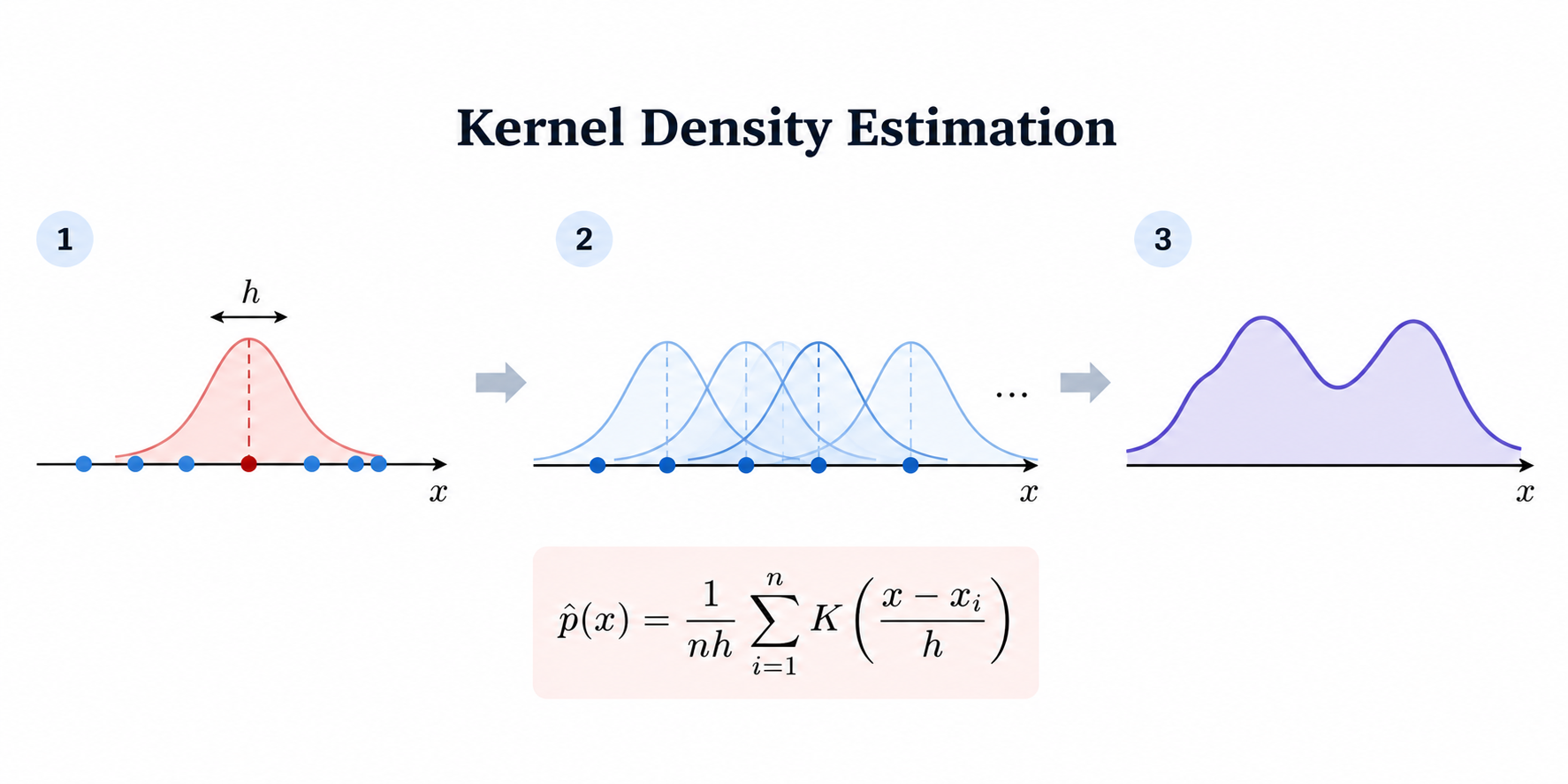
Interestingly, the kernel can also be interpreted as a probability distribution:
\[K_{\sigma}(u) \geq 0, \qquad \int K_{\sigma}(u)\,du = 1.\]Under this interpretation, the smoothed data distribution is
\[p_{\sigma}(x) = \int_{x'} p_{\sigma}(x\mid x')p(x')dx'.\]A common choice is the Gaussian kernel. In one dimension,
\[K_{\sigma}(x-x')=\frac{1}{\sigma \sqrt{2\pi}}\exp\left(-\frac{(x-x')^2}{2\sigma^2}\right),\]or equivalently,
\[p_{\sigma}(x\mid x')=\mathcal{N}(x;x',\sigma^2),\]where $\mathcal{N}(x;x',\sigma^2)$ denotes the Gaussian density evaluated at $x$, with mean $x'$ and variance $\sigma^2$.
As $\sigma\to0$, the smoothed distribution approaches the original data distribution:
\[\lim_{\sigma\to0} p_{\sigma}(x) = p(x).\]Therefore, we can approximate the original score by learning the score of a smoothed distribution.
Now, let us compute the score of $p_{\sigma}(x)$:
\[\begin{align} \nabla \log p_{\sigma}(x) &= \frac{\nabla p_{\sigma}(x)}{p_{\sigma}(x)}\\ &= \int_{x'} \frac{p(x')}{p_{\sigma}(x)} \nabla p_{\sigma}(x\mid x') dx'\\ &= \int_{x'} \frac{p_{\sigma}(x\mid x')p(x')}{p_{\sigma}(x)} \nabla \log p_{\sigma}(x\mid x') dx'. \end{align}\]Notice that the fraction in the final expression is precisely the posterior distribution $p_{\sigma}(x'\mid x)$. In other words, the score of the smoothed distribution is the posterior expectation of the conditional score:
\[\nabla\log p_{\sigma}(x) = \mathbb{E}_{p_{\sigma}(x'\mid x)} \left[\nabla\log p_{\sigma}(x\mid x')\right].\]For a Gaussian kernel, the conditional score has a simple closed form:
\[\nabla_x\log p_{\sigma}(x\mid x') = \frac{x'-x}{\sigma^2}.\]This gives us a practical training objective:
\[\min_{\theta} \mathbb{E}_{x\sim p_{\sigma}(x\mid x'),\,x'\sim p(x')} \left[ \left\Vert s_{\theta}(x)-\frac{x'-x}{\sigma^2}\right\Vert^2 \right].\]The key insight is that we no longer need to know the original density or its score. We only need to sample a clean data point $x'$, perturb it with Gaussian noise to obtain $x$, and train the network to predict the direction back toward the clean sample.
Although each individual target points toward one particular data point, minimizing the expected MSE recovers the score of the smoothed distribution. This is known as denoising score matching.
Finally, the choice of $\sigma$ matters. A smaller $\sigma$ produces a more accurate approximation of the original distribution, but it also makes score estimation difficult in low-density regions, where very few samples contribute meaningfully to the estimate.
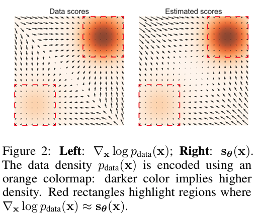
To address this issue, Song & Ermon propose learning scores at multiple noise levels:
\[\sigma_T > \sigma_{T-1} > \cdots > \sigma_1.\]At each noise level, we learn the score of the corresponding perturbed data distribution $p_{\sigma_t}(x)$.
When $\sigma$ is large, the perturbed distribution can differ substantially from the original data distribution. Rather than directly sampling using the score at the smallest noise level, we can gradually transition through a sequence of increasingly less noisy distributions.
Specifically, we start from a high-noise distribution, apply several Langevin steps at the current noise level, and use the resulting sample to initialize the next, smaller noise level. This procedure is known as annealed Langevin dynamics:
\[x_t^{(k+1)} = x_t^{(k)} + \frac{\sigma_t^2}{2} \nabla \log p_{\sigma_t}\left(x_t^{(k)}\right) + \sigma_t\,\xi^{(k)}, \qquad \xi^{(k)} \sim \mathcal{N}(0,I), \qquad t=1,\cdots,T.\]Here, we run several Langevin steps $k=0,\cdots,K-1$ at each noise level, then initialize the next level with the final sample:
\[x_{t}^{(0)} = x_{t+1}^{(K)}.\]The sampling process therefore progressively transitions through
\[p_{\sigma_T}(x), p_{\sigma_{T-1}}(x), \ldots, p_{\sigma_1}(x),\]eventually approaching the original data distribution as $\sigma_1\to0$, assuming the sampling process sufficiently tracks these intermediate distributions.
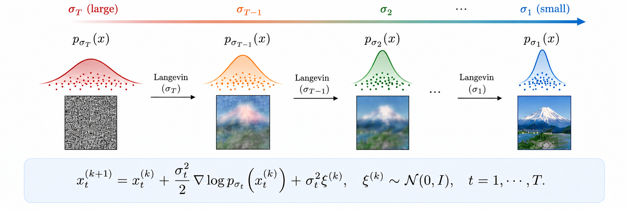
This reveals the connection to diffusion models: both construct a generative process that progressively transforms noise into data through a sequence of intermediate distributions.
Conceptually, diffusion models take this annealed sampling idea further by learning transitions that progressively remove noise. However, standard reverse diffusion updates are not literally equivalent to taking annealed Langevin dynamics with $K=1$.
Neural Langevin Dynamics
Now, back to our main theme of unsupervised diffusion training. Given only an energy-based target distribution, can we perform Langevin-like sampling without explicitly learning its score?
The key is an optimization-based reinterpretation of Langevin dynamics. Recall the standard update:
\[x' = x+ \frac{\sigma^2}{2}\nabla_x \log p(x) + \sigma\,\xi, \qquad \xi\sim\mathcal N(0,I).\]Instead of viewing this merely as a stochastic gradient update, we can characterize its transition distribution $p(x'\mid x)$ as the solution to a local optimization problem:
\[\begin{aligned} \min_{p(x'\mid x)} \left\{ \frac{1}{2} \mathbb{E}_{p(x'\mid x)} \left[ -\nabla_x\log p(x)^\top(x'-x) \right] + D_{\mathrm{KL}} \left( p(x'-x\mid x) \,\middle\|\, \mathcal N(0,\sigma^2 I) \right) \right\}. \end{aligned}\]To see why, recall that minimizing an expected cost plus a KL divergence produces a distribution proportional to the reference distribution multiplied by the exponential of the negative cost. Here, the resulting distribution is
\[p^*(x'-x\mid x) \propto \mathcal N(x'-x;0,\sigma^2 I) \exp\left( \frac{1}{2}\nabla_x\log p(x)^\top(x'-x) \right),\]which is precisely
\[p^*(x'\mid x) = \mathcal N\left( x'; x+\frac{\sigma^2}{2}\nabla_x\log p(x), \sigma^2 I \right).\]Thus, the Langevin update can be recovered by solving a local KL-regularized optimization problem. This is closely related to the optimization view of a single gradient-descent step: we seek an update that improves the objective while regularizing how far the update can move.
We can take this interpretation one step further. By a first-order Taylor approximation,
\[-\nabla_x\log p(x)^\top(x'-x) \approx \log p(x)-\log p(x').\]Since $\log p(x)$ is constant with respect to $x'$, the local Langevin objective can be approximated by
\[\boxed{ \min_{p(x'\mid x)} \left\{ \frac{1}{2} \mathbb{E}_{p(x'\mid x)} \left[-\log p(x')\right] + D_{\mathrm{KL}} \left( p(x'-x\mid x) \,\middle\|\, \mathcal N(0,\sigma^2 I) \right) \right\}. }\]This gives a particularly intuitive interpretation of a Langevin step:
- Move toward a higher-probability state: minimizing $-\log p(x')$ encourages the next state to have higher probability under the target distribution.
- Keep the update local: the KL regularization constrains the update distribution around a Gaussian perturbation, keeping the local approximation meaningful.
Importantly, the second objective/distribution is a more generalized version of the original Langevin update, which is known as locally-balanced proposal.
This perspective is useful because it allows us to move beyond explicitly estimating the score $\nabla_x\log p(x)$ and instead directly optimize a parameterized transition distribution:
\[\min_{\theta} \left\{ \frac{1}{2} \mathbb{E}_{p_\theta(x'\mid x)} \left[-\log p(x')\right] + D_{\mathrm{KL}} \left( p_\theta(x'-x\mid x) \,\middle\|\, \mathcal N(0,\sigma^2 I) \right) \right\}.\]For our energy-based target, we have
\[-\log p(x') = \frac{g(x')}{\beta}+\mathrm{const.}\]Therefore, the expected target cost becomes
\[\mathbb{E}_{p_\theta(x'\mid x)} [-\log p(x')] = \mathbb{E}_{p_\theta(x'\mid x)} \left[\frac{g(x')}{\beta}\right] +\mathrm{const.}\]If this expectation cannot be differentiated through $x'$, its gradient can again be estimated using REINFORCE.
Importantly, the objective is local to a single transition. Rather than propagating a terminal reward backward through an entire generation trajectory, we can directly optimize each transition using the energy of its next state.
More generally, this local optimization perspective is not restricted to isotropic Gaussian transitions. We can introduce different reference distributions $p_{\mathrm{ref}}(x'\mid x)$ and constraints to control how each step explores the state space. For example, in my work on Regularized Langevin Dynamics, I constrain the update magnitude in the combinatorial space to encourage exploration, which I will discuss in future blog posts.
In simple words, Langevin dynamics decouples long-horizon generation from local transition optimization. Rather than directly optimizing an entire generation trajectory, we can repeatedly solve, or learn, a simpler per-step objective. This perspective not only makes optimization easier to handle, but also gives us considerable freedom to design different local update rules, regularizers, and exploration mechanisms for different state spaces and generation problems.
Perspective 2: Chain of Latent Variables
Let us now revisit diffusion models from a different perspective: a chain of latent variables, as introduced in the original DDPM paper.

Assume we have a data distribution $p_{\mathrm{data}}(x)$. We define a forward process that gradually adds noise to the data:
\[x_0 \to x_1 \to \cdots \to x_T,\]where each transition follows a Gaussian distribution:
\[q(x_t\mid x_{t-1}) = \mathcal{N}\left( x_t;\sqrt{1-\beta_t}x_{t-1},\beta_t I \right).\]The reverse process, or generation process, aims to reverse this chain, starting from noise $x_T$ and eventually generating a clean sample $x_0$.
Our ultimate goal is to match the generated distribution to the data distribution:
\[\min_\theta D_{\mathrm{KL}}(p_{\mathrm{data}}(x_0)\|p_\theta(x_0)).\]However, directly evaluating the marginal distribution
\[p_\theta(x_0) = \int_{x_{1:T}}p_\theta(x_{0:T})\,dx_{1:T}\]is generally intractable.
The key idea is to lift the objective from the marginal distribution to the joint distribution over the entire trajectory. By the data-processing inequality,
\[D_{\mathrm{KL}}(p_{\mathrm{data}}(x_0)\|p_\theta(x_0)) \leq D_{\mathrm{KL}}(p(x_{0:T})\|p_\theta(x_{0:T})),\]where
\[p(x_{0:T}) = p_{\mathrm{data}}(x_0) \prod_{t=1}^Tq(x_t\mid x_{t-1}),\]and
\[p_\theta(x_{0:T}) = p(x_T) \prod_{t=1}^Tp_\theta(x_{t-1}\mid x_t).\]Intuitively, matching the entire trajectory is a stronger requirement than matching only its final output. Therefore, minimizing the joint KL also minimizes an upper bound on the marginal KL.
More importantly, the joint KL can be decomposed into tractable terms:
\[\begin{aligned} &D_{\mathrm{KL}}\left(p(x_{0:T})\,\|\,p_\theta(x_{0:T})\right) \\ =&\; \underbrace{ \mathbb{E}_{p_{\mathrm{data}}(x_0)} \left[ D_{\mathrm{KL}}\left(q(x_T\mid x_0)\,\|\,p(x_T)\right) \right] }_{L_T} \\ &+ \sum_{t=2}^{T} \underbrace{ \mathbb{E}_{q(x_0,x_t)} \left[ D_{\mathrm{KL}}\left( q(x_{t-1}\mid x_t,x_0) \,\|\, p_\theta(x_{t-1}\mid x_t) \right) \right] }_{L_{t-1}} \\ &+ \underbrace{ -\mathbb{E}_{q(x_0,x_1)} \left[\log p_\theta(x_0\mid x_1)\right] }_{L_0} +\mathrm{const.} \end{aligned}\]Therefore, ignoring terms independent of $\theta$, the DDPM training objective is
\[\boxed{ L_{\mathrm{DDPM}} = L_0+\sum_{t=1}^{T-1}L_t+L_T. }\]Here, our derivation differs slightly from the ELBO derivation in the original DDPM paper, but the resulting objective is equivalent. The advantage of this data-processing perspective is that it applies equally well when we reverse the direction of the KL divergence, as we will see shortly.
Now, let us return to our main question:
What if we do not have samples from the target distribution, but only an energy function?
Forward KL
The forward KL requires samples from the target distribution. Without access to such samples, can we still use this objective?
Yes, through sampling methods from the previous blog post.
The idea is to first approximate samples from the energy-based target distribution using importance sampling (IS), sequential Monte Carlo (SMC), MCMC, or related methods, and then train the diffusion model using a weighted version of the standard DDPM objective.
Let us use importance sampling version as an example.
Recall that our target distribution is
\[\begin{align} p(x_{0:T})&\propto p_{\mathrm{ref}}(x_{0:T})\exp\left(-\frac{g(x_0)}{\beta}\right)\\ &\propto\prod_{t=1}^Tq(x_t\mid x_{t-1})\exp\left(-\frac{g(x_0)}{\beta}\right), \end{align}\]We then use the current diffusion model as the proposal distribution. Specifically:
-
Generate samples: Sample $N$ trajectories $\lbrace x^i_{0:T}\rbrace_{i=1}^N$ from the current model $p_\theta(x_{0:T})$.
-
Compute importance weights: For each trajectory, evaluate its unnormalized importance weight:
- Normalize the weights:
- Train the model: Use the weighted samples to approximate the expectation under the target trajectory distribution. The resulting training objective is
where $L_{\mathrm{DDPM}}(x_0^i)$ denotes the standard DDPM loss evaluated using the forward noising process conditioned on $x_0^i$.
During each optimization step, we treat the importance weights and sampled trajectories as fixed when differentiating the weighted training objective.
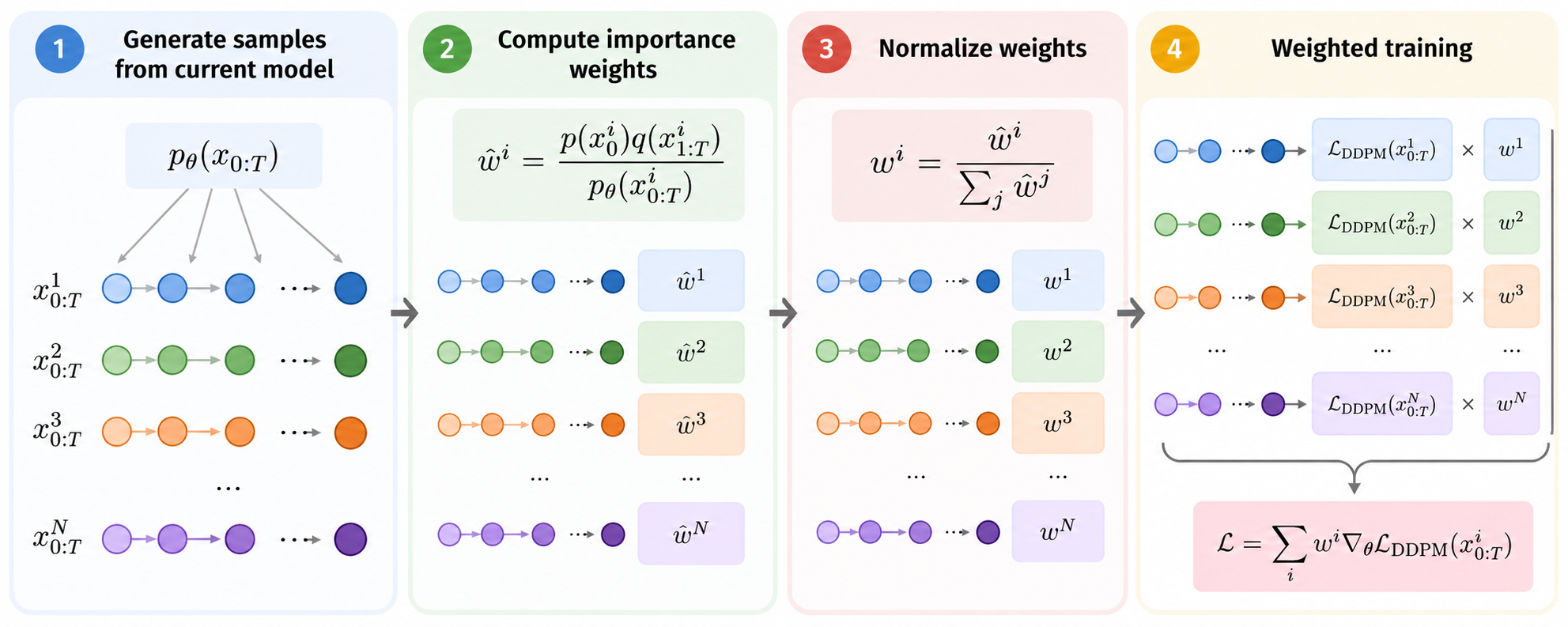
The intuition is simple: we generate samples from our current model, assign higher weights to trajectories that are more representative of the target distribution, and use them to train the diffusion model.
In principle, this allows us to optimize the forward KL without direct access to samples from the target distribution.
However, importance sampling becomes increasingly difficult in high-dimensional spaces. Most trajectories may receive negligible weights, leaving only a few effective training samples.
This motivates a different approach: reverse KL.
Reverse KL
Unlike the forward KL, the reverse KL takes its expectation under the model distribution:
\[\min_\theta D_{\mathrm{KL}}(p_\theta(x_0)\|p(x_0)).\]This is particularly appealing for unsupervised diffusion training because we can sample from our model, even when we cannot sample directly from the target distribution.
As before, we can apply the data-processing inequality to obtain an upper bound by lifting the KL to the trajectory space:
\[D_{\mathrm{KL}}(p_\theta(x_0)\|p(x_0)) \leq D_{\mathrm{KL}}(p_\theta(x_{0:T})\|p(x_{0:T})).\]Expanding the joint KL gives
\[\boxed{ \begin{aligned} &D_{\mathrm{KL}}\left( p_\theta(x_{0:T})\,\|\,p(x_{0:T}) \right) \\ =& \underbrace{ -\sum_{t=1}^{T} \mathbb{E}_{p_\theta(x_{t:T})} \left[ \mathcal{H}\left( p_\theta(x_{t-1}\mid x_t) \right) \right] }_{L_{\mathrm{entropy}}} \\ &+ \underbrace{ -\sum_{t=1}^{T} \mathbb{E}_{p_\theta(x_{t-1:T})} \left[ \log q(x_t\mid x_{t-1}) \right] }_{L_{\mathrm{forward}}} \\ &+ \underbrace{ -\mathbb{E}_{p_\theta(x_{0:T})} \left[ \log p(x_0) \right] }_{L_{\mathrm{target}}} +\mathrm{const.} \end{aligned}}\]Here, we have absorbed the fixed prior term involving $p(x_T)$ into the constant, assuming the initial noise distribution of the reverse process is fixed.
Recall that
\[\log p(x_0) = -\frac{g(x_0)}{\beta}+\mathrm{const.}\]The resulting objective has three intuitive components:
-
$L_{\mathrm{entropy}}$ — Encourage exploration. Maximizing the entropy of each reverse transition prevents the model from becoming overly deterministic, analogous to entropy regularization in soft RL.
-
$L_{\mathrm{forward}}$ — Regularize the transitions. Maximizing the likelihood under the forward noising process encourages consecutive states to remain compatible with the prescribed noise schedule. For Gaussian transitions, this corresponds to a quadratic penalty on the difference between consecutive states, after accounting for the forward-process mean and variance.
-
$L_{\mathrm{target}}$ — Optimize the final sample. Minimizing $-\log p(x_0)$ is equivalent to minimizing the energy $g(x_0)$, encouraging the generated samples to concentrate in high-probability regions of the target distribution.
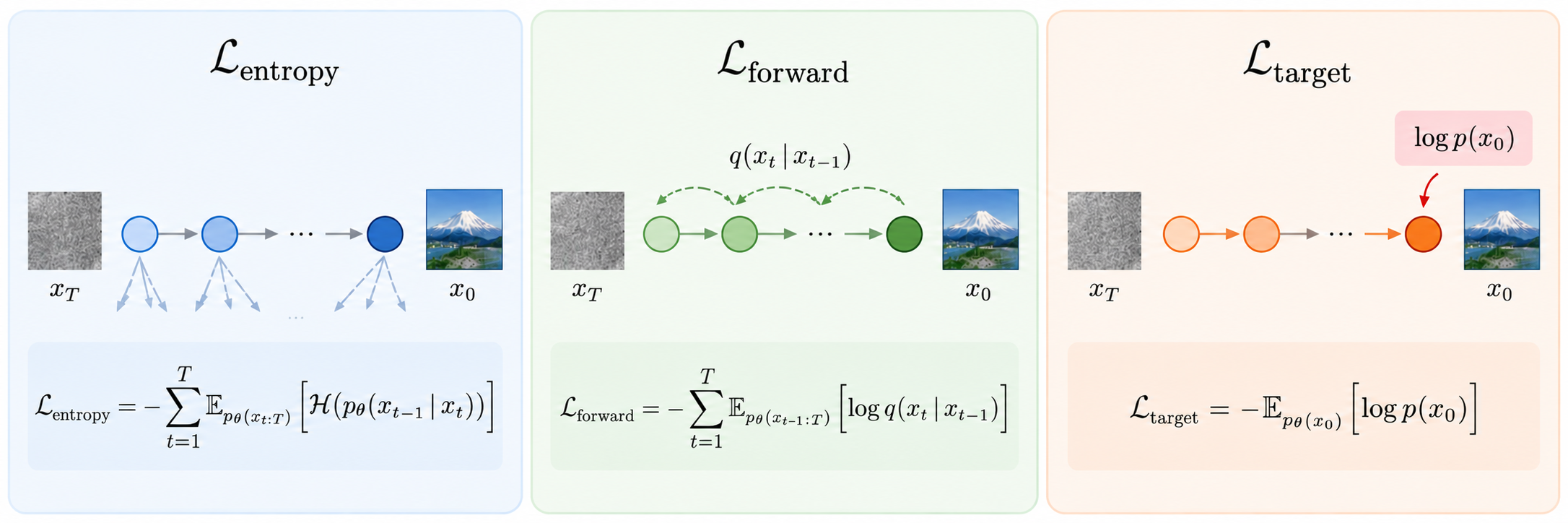
In other words, reverse KL combines exploration, transition regularization, and final-sample optimization into a single objective.
However, optimizing this objective is not straightforward — we need to differentiate terms like $g(x_0)$ against the prior states.
One general solution is to use policy-gradient methods such as REINFORCE, as explored by Sanokowski et al., 2024. However, this brings us back to the familiar challenges of reinforcement learning: high-variance gradient estimates and credit assignment across a long generation trajectory.
Can we instead exploit the structure of the continuous-time diffusion process to optimize the generation trajectory more directly?
This brings us to our final perspective.
Perspective 3: Stochastic Differential Equations (SDEs)
Our final perspective is perhaps the most powerful one: viewing diffusion models as continuous-time stochastic processes.
When the step size becomes sufficiently small, the iterative generation process can be described by a stochastic differential equation (SDE). As discussed by Song et al., both the forward noising process and the reverse generation process can be expressed through SDEs:
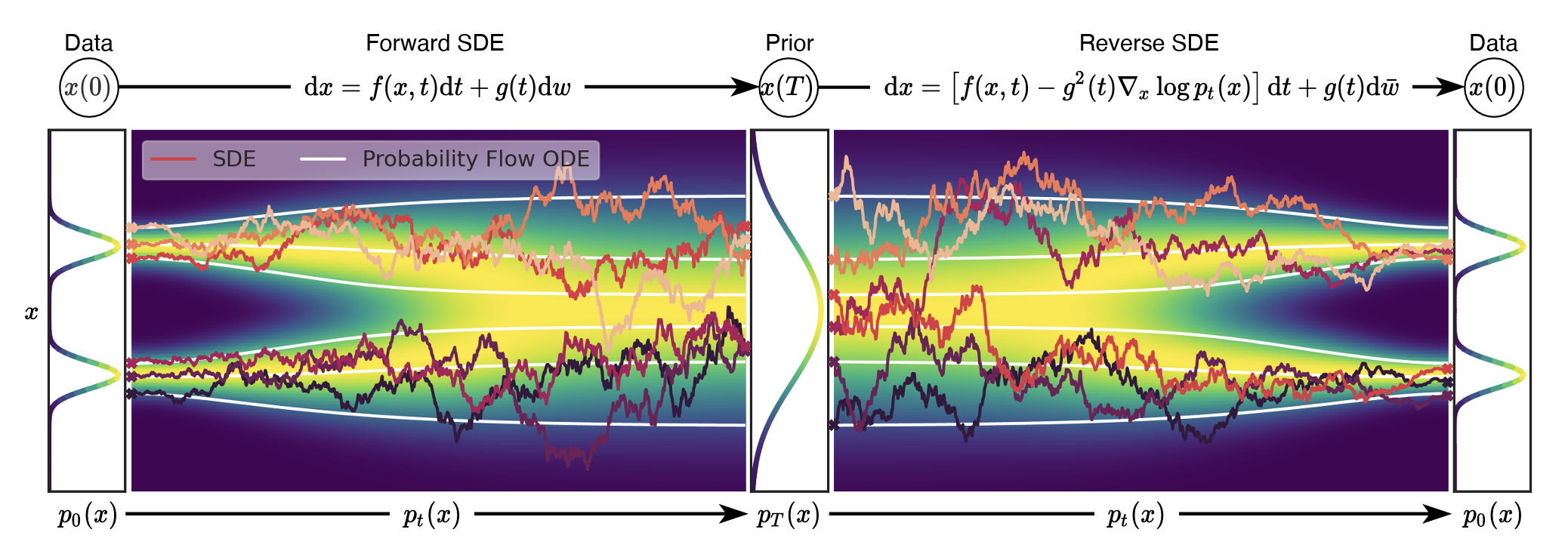
A closely related continuous-time perspective is flow matching, which learns a deterministic ordinary differential equation (ODE) that transports samples between probability distributions.
In this section, we will focus on the SDE formulation and show how stochastic optimal control provides a natural framework for training diffusion models using only an energy-based target.
Stochastic Optimal Control
Let us start with the simplest possible SDE:
\[dx_t = \sigma_t\,dw_t,\]where $w_t$ denotes standard Brownian motion and $\sigma_t$ controls the magnitude of the injected Gaussian noise. The noise schedule $\sigma_t$ is typically specified in advance.
Without any additional drift, the particle simply performs a random walk in space. There is nothing guiding it toward our desired target distribution.
We denote the resulting trajectory distribution by $p_{\mathrm{ref}}(x_{0:1})$, which serves as our reference process.
Now, suppose we want to steer the particle toward regions with low cost or high reward. We can introduce a learnable control $u_\theta(x_t,t)$ that guides its movement:
\[dx_t = \sigma_t u_\theta(x_t,t)\,dt + \sigma_t\,dw_t.\]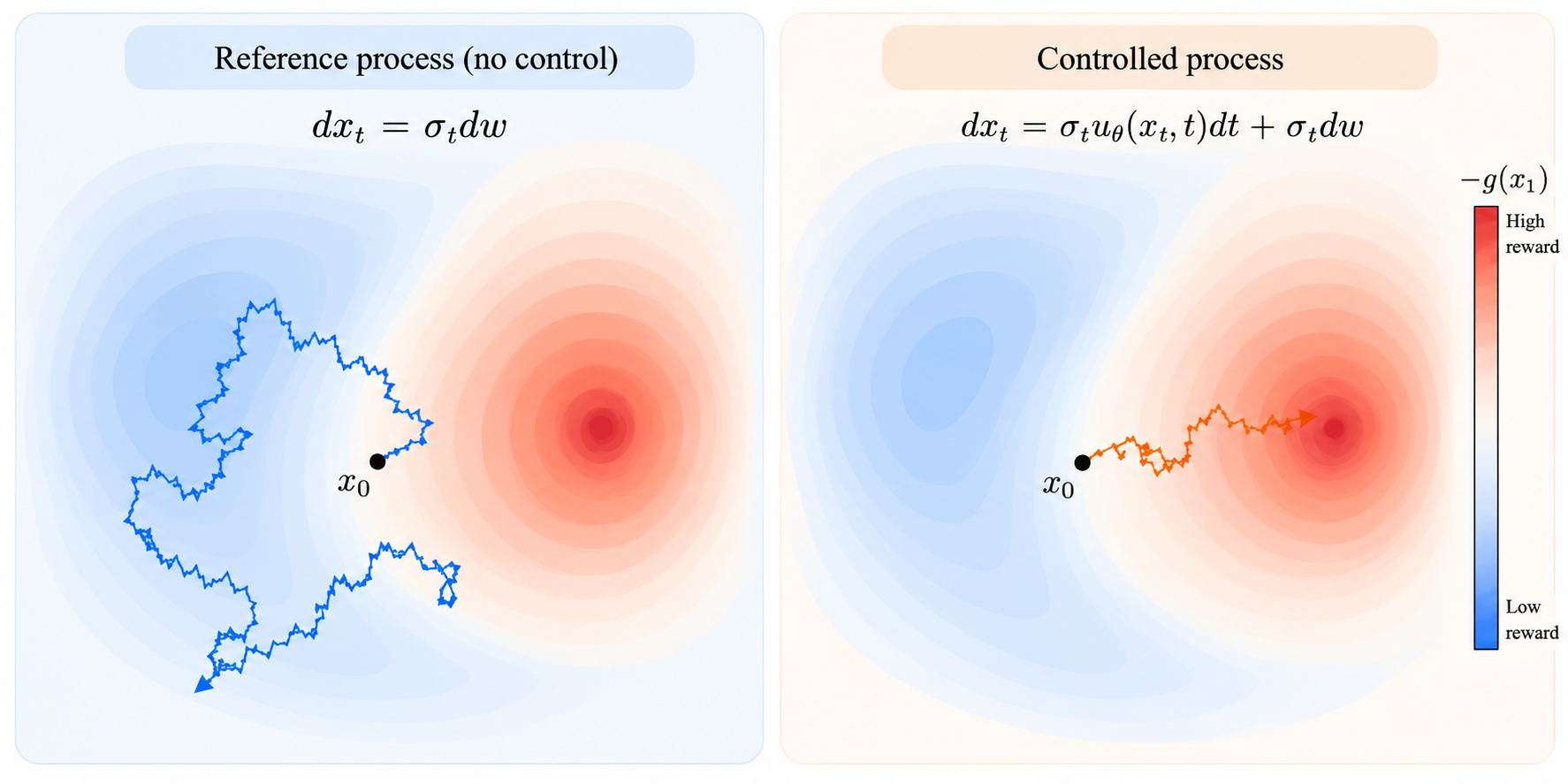
The control changes the trajectory distribution from $p_{\mathrm{ref}}(x_{0:1})$ to $p_{u_\theta}(x_{0:1})$.
Naturally, we would like to minimize the expected terminal cost while preventing the controlled process from deviating too far from the reference process. This leads to the stochastic optimal control (SOC) objective:
\[\boxed{ \min_\theta J(u_\theta) = D_{\mathrm{KL}}\left( p_{u_\theta}(x_{0:1}) \|p_{\mathrm{ref}}(x_{0:1}) \right) + \mathbb{E}_{u_\theta}\left[\frac{g(x_1)}{\beta}\right]. }\]Here, we assume that the controlled and reference processes share the same initial distribution and diffusion coefficient.
By the Girsanov theorem, the trajectory-level KL divergence can be expressed as the expected squared control:
\[D_{\mathrm{KL}}\left( p_{u_\theta}(x_{0:1}) \|p_{\mathrm{ref}}(x_{0:1}) \right) = \frac12 \mathbb{E}_{u_\theta} \left[ \int_0^1 \|u_\theta(x_t,t)\|^2dt \right].\]Therefore, the SOC objective becomes
\[\boxed{ \min_\theta J(u_\theta) = \mathbb{E}_{u_\theta} \left[ \int_0^1 \frac12\|u_\theta(x_t,t)\|^2dt + \frac{g(x_1)}{\beta} \right]. }\]The integral term is often interpreted as the kinetic energy or control effort of the process. It has two intuitive implications:
- Prefer small control: Large deviations from the reference dynamics incur a higher cost. For a simple Brownian reference process, this discourages unnecessarily large or rapidly changing movements.
- Distribute control across time: Because the cost is quadratic, applying a large control over a short interval is generally more expensive than distributing the same total displacement over a longer interval.
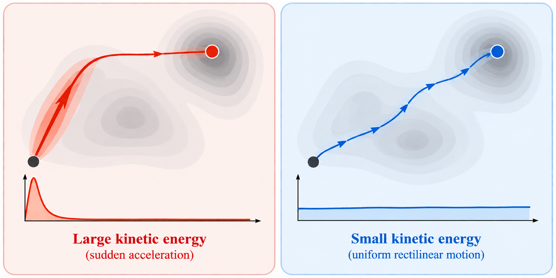
Interestingly, the SOC objective closely resembles the reverse KL objective derived in Perspective 2. We can establish the following conceptual correspondence:
| Reverse KL (Discrete-time) | Stochastic Optimal Control (Continuous-time) | Interpretation |
|---|---|---|
| $L_{\mathrm{entropy}}$ | Included in the path-space KL | Encourages stochastic exploration |
| $L_{\mathrm{forward}}$ | Included in $\frac12\mathbb{E}_{u_\theta}[\int_0^1\Vert u_\theta(x_t,t)\Vert^2dt]$ | Regularizes deviations from the reference process |
| $L_{\mathrm{target}}$ | $\mathbb{E}_{u_\theta}[g(x_1)/\beta]$ | Encourages high-quality final samples |
Under compatible reference dynamics and discretization assumptions, the discrete-time path-space KL converges to the corresponding continuous-time control cost.
We can also generalize the reference process by introducing a pretrained drift $u_{\mathrm{ref}}(x_t,t)$:
\[dx_t = \sigma_t u_{\mathrm{ref}}(x_t,t)\,dt + \sigma_t\,dw_t.\]If the controlled process uses $u_\theta(x_t,t)$ as its total drift coefficient, the KL regularization becomes
\[\frac12 \mathbb{E}_{u_\theta} \left[ \int_0^1 \|u_\theta(x_t,t)-u_{\mathrm{ref}}(x_t,t)\|^2dt \right].\]The interpretation is straightforward: we penalize the additional control required to deviate from the pretrained dynamics, rather than penalizing the entire drift.
Adjoint Method
Establishing the SOC formulation does not directly resolve the optimization challenge we encountered with the reverse KL objective: how can we propagate the terminal cost through a long stochastic generation trajectory efficiently?
This is where the adjoint method comes into play.
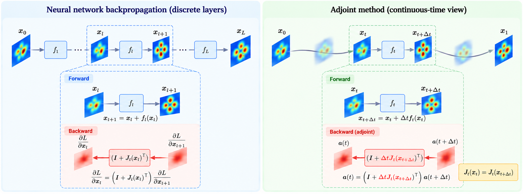
At a high level, the adjoint method can be understood as backpropagation extended to continuous-time dynamics, with the additional advantage that intermediate states can sometimes be reconstructed by integrating backward rather than storing every state.
To build some intuition, consider a residual neural network layer:
\[x_{l+1}=x_l+f_l(x_l).\]The backward recursion is
\[\frac{\partial L}{\partial x_l} = \left( I+\nabla_x f_l(x_l) \right)^\top \frac{\partial L}{\partial x_{l+1}}.\]Standard backpropagation typically stores intermediate activations $x_l$ to evaluate the Jacobian $\nabla_x f_l(x_l)$.
Now consider a continuous-time ODE:
\[\frac{dx_t}{dt}=f(x_t,t).\]Its discretized forward update is
\[x_{t+\Delta t} = x_t+f(x_t,t)\Delta t.\]The corresponding backward recursion is approximately
\[\frac{\partial L}{\partial x_t} = \left( I+\Delta t\,\nabla_x f(x_t,t) \right)^\top \frac{\partial L}{\partial x_{t+\Delta t}}.\]As $\Delta t\to0$, this becomes a continuous-time backward differential equation.
The important computational difference is that, for a sufficiently well-behaved invertible ODE flow, we can reconstruct intermediate states by solving the dynamics backward in time, rather than storing every forward activation.
This gives the adjoint method its potential memory advantage, although numerical reconstruction can introduce errors and stochastic trajectories require additional care.
Now let us return to our SOC objective:
\[J(u) = \mathbb{E}_u \left[ \int_0^1 \frac12\|u(x_t,t)\|^2dt + \frac{g(x_1)}{\beta} \right].\]For simplicity, we write $u$ instead of $u_\theta$ when discussing the control function.
Given a trajectory $x_{0:1}$ generated under control $u$, we define the adjoint $a(t)$ as the sensitivity of the remaining trajectory cost to the current state:
\[a(t) = \nabla_{x_t} \left( \int_t^1 \frac12\|u(x_\tau,\tau)\|^2d\tau + \frac{g(x_1)}{\beta} \right),\]where the gradient is taken through the future trajectory while holding the future Brownian increments fixed.
For our controlled dynamics
\[dx_t = \sigma_t u(x_t,t)\,dt+\sigma_t\,dw_t,\]the adjoint satisfies the backward ODE
\[\frac{d}{dt}a(t) = -\left[ \sigma_t (\nabla_x u(x_t,t))^\top a(t) + \nabla_x\left( \frac12\|u(x_t,t)\|^2 \right) \right],\]with terminal condition
\[a(1)= \frac{\nabla_x g(x_1)}{\beta}.\]The adjoint tells us how much the remaining cost would change if we slightly perturbed the current state.
But how does this give us the gradient with respect to the control?
Recall that the control affects the state dynamics through $\sigma_t u(x_t,t)$. Over a small time interval $\Delta t$, a perturbation $\delta u$ changes the next state by approximately
\[\delta x_{t+\Delta t} \approx \sigma_t\delta u\,\Delta t.\]Therefore, by the chain rule, the contribution of the future cost to the control gradient is $\sigma_t a(t)$ per unit time.
Combining this with the immediate control cost, we obtain
\[\boxed{ \nabla_{u(x_t,t)}J = u(x_t,t)+\sigma_t a(t), }\]where this expression represents the trajectory-wise functional-gradient contribution, before taking the appropriate expectation over trajectories.
This motivates the following objective:
\[\boxed{ \mathcal{L}_{\mathrm{adjoint}} = \frac12 \int_0^1 \left\| u_\theta(x_t,t) + \sigma_t a(t) \right\|^2dt. }\]Here, the sampled trajectory and adjoint target are treated as fixed when differentiating the regression loss with respect to $\theta$.
In other words, the adjoint allows us to compute the gradient of the future cost with respect to the control by propagating sensitivity backward through the trajectory.
However, computing the adjoint still requires evaluating the Jacobian $\nabla_x u(x_t,t)$ at every time step, which can be prohibitively expensive for large neural networks.
This motivates a further simplification.
Adjoint Matching
The key observation behind Adjoint Matching is that the optimal control satisfies a special consistency condition.
Recall that the optimal control must balance the immediate control cost against its effect on the expected future cost:
\[\boxed{ u^*(x_t,t) + \sigma_t \mathbb{E}_{u^*} \left[ a(t)\mid x_t \right] =0. }\]This is the first-order optimality condition for the control.
Optional: An intuitive derivation of the optimality condition
Let us first define the optimal future cost:
\[V_t(x) = \min_u \mathbb{E}_u \left[ \int_t^1 \frac12\|u(x_\tau,\tau)\|^2d\tau + g(x_1) \mid x_t=x \right].\]The control at time $t$ affects two terms in our objective:
- Immediate cost: $\frac12\Vert u(x_t,t)\Vert^2\Delta t$.
- Future cost: $\mathbb{E}_{x'}[V_{t+\Delta t}(x')]$.
Combining these terms, we have
\[J_t(u) = \frac12\|u(x_t,t)\|^2\Delta t + \mathbb{E}_{x'}[V_{t+\Delta t}(x')].\]At the optimum, $\nabla_u J_t(u)=0$.
To compute this gradient, recall that the state transition follows
\[x' = x_t + \sigma_t u(x_t,t)\Delta t + \sigma_t\sqrt{\Delta t}\,\epsilon, \qquad \epsilon\sim\mathcal N(0,I).\]By the chain rule,
\[\begin{aligned} \nabla_u \mathbb{E}[V_{t+\Delta t}(x')] &= \mathbb{E}_{\epsilon} \left[ \nabla_u V_{t+\Delta t}(x') \right] \\ &= \sigma_t\Delta t\, \mathbb{E}_{\epsilon} \left[ \nabla_{x'}V_{t+\Delta t}(x') \right]. \end{aligned}\]As $\Delta t\to0$, assuming sufficient smoothness,
\[\mathbb{E}_{\epsilon} \left[ \nabla_{x'}V_{t+\Delta t}(x') \right] \to \nabla_{x_t}V_t(x_t).\]Substituting this into $\nabla_u J_t(u)=0$, we obtain
\[\begin{aligned} &u(x_t,t)\Delta t + \sigma_t\Delta t\, \nabla_{x_t}V_t(x_t) + o(\Delta t) =0 \\ \Rightarrow\quad& \boxed{ u^*(x_t,t) = -\sigma_t\nabla_{x_t}V_t(x_t). } \end{aligned}\]This is the optimal control condition.
Since the gradient of the value function equals the conditional expectation of the trajectory adjoint at optimality,
\[\nabla_{x_t}V_t(x_t) = \mathbb{E}_{u^*} \left[ a(t)\mid x_t \right],\]we recover
\[\boxed{ u^*(x_t,t) + \sigma_t \mathbb{E}_{u^*} \left[ a(t)\mid x_t \right] =0. }\]Now, let us examine what this condition implies for the backward adjoint equation.
Multiplying the optimality condition by the Jacobian $\nabla_x u^*(x_t,t)$ gives
\[\mathbb{E}_{u^*} \Big[ \sigma_t (\nabla_x u^*(x_t,t))^\top a(t) + \nabla_x \left( \frac12\|u^*(x_t,t)\|^2 \right) \mid x_t \Big] =0.\]Notice that the expression inside the expectation is exactly the term appearing in the backward ODE of the full adjoint.
Therefore, at optimality, the conditional expectation of the full adjoint's drift vanishes.
This does not mean that $a(t)$ is constant along every stochastic trajectory. Instead, it suggests that these terms can be removed when constructing a simpler regression target, without changing the desired optimal control.
This leads to the lean adjoint $\tilde a(t)$, whose backward ODE contains only the derivatives of the uncontrolled reference drift and any additional running state cost.
In our simple Brownian reference setup, both are zero, so
\[\frac{d}{dt}\tilde a(t)=0,\]with terminal condition
\[\tilde a(1)=\frac{\nabla_x g(x_1)}{\beta}.\]Therefore,
\[\boxed{ \tilde a(t) = \frac{\nabla_x g(x_1)}{\beta}. }\]The resulting Adjoint Matching objective is remarkably simple:
\[\boxed{ \mathcal{L}_{\mathrm{AM}} = \frac12 \int_0^1 \left\| u_\theta(x_t,t) + \frac{\sigma_t}{\beta}\nabla_x g(x_1) \right\|^2dt. }\]Again, the sampled trajectory and the terminal-gradient target are treated as fixed when differentiating this regression objective.
How should we understand this objective?
Formally, it is a regression-based fixed-point formulation of optimal control. Under the assumptions of the Adjoint Matching analysis, the optimal control is the unique critical point of the expected regression objective when the sampling distribution and targets are updated consistently with the current control.
My personal takeaway is more intuitive: we use the desired update at the terminal state to guide the control at every intermediate state.
Rather than explicitly backpropagating the terminal cost through the entire neural network at every diffusion step, we match each local control against a target constructed from the terminal gradient.
This interpretation is especially useful when extending adjoint matching to other settings, including discrete state spaces.
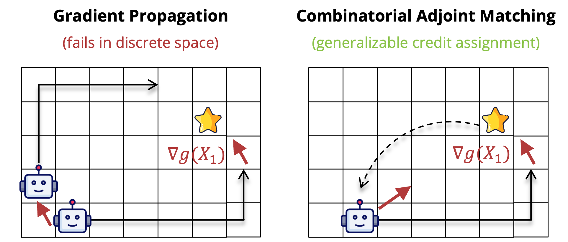
In my earlier work, I developed Combinatorial Adjoint Matching (CAM), which extends this idea to combinatorial optimization while addressing the non-differentiability of discrete transitions. The high-level idea is illustrated below:
The final question:
How can we obtain $\nabla g(x_1)$?
I list several practices:
- The simplest case is that $g(\cdot)$ itself is differentiable, like a neural network or a differentiable objective;
- If there is some local search heuristic, we can rely on it to find the locally improved solution, like used in CAM;
- REINFORCE is another option, as introduced by RAM.
- Finally, similar to forward KL, we can rely on the sampling method to estimate the optimal control, as tried by DAM.
Case Study (Maximum Independent Set)
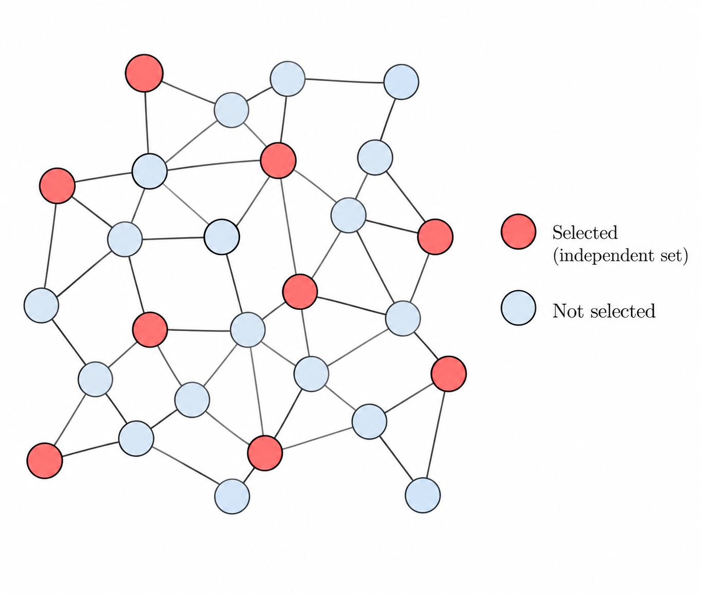
As a concrete example, let us consider Maximum Independent Set (MIS), a classical combinatorial optimization problem. Given a graph $G=(V,E)$, our goal is to select as many vertices as possible without selecting any two connected vertices.
MIS admits a simple quadratic objective over binary variables $x_i\in\lbrace0,1\rbrace$, where $x_i=1$ indicates that vertex $i$ is selected:
\[\boxed{ \min_{x\in\{0,1\}^{|V|}} g(x) = -\sum_{i\in V}x_i + \lambda\sum_{(i,j)\in E}x_ix_j, }\]where $\lambda>1$ penalizes selecting adjacent vertices. Despite its simple objective and strong local structure, MIS remains a challenging discrete optimization problem.
Below, we compare the different diffusion training approaches discussed in this blog:
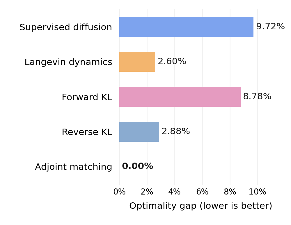
The results suggest that for problems with strong local structure, supervised diffusion from optimal solutions is not necessarily superior to unsupervised training. In particular, Langevin-based methods can achieve competitive performance by exploiting local information from the objective, while adjoint matching achieves the lowest optimality gap among the compared methods.
This reinforces our central takeaway: the structure of diffusion processes offers opportunities for efficient unsupervised training beyond general-purpose reinforcement learning methods.
Conclusion
We have explored three perspectives on diffusion models, each offering a different approach to unsupervised training:
- Langevin Dynamics: Decomposes global trajectory optimization into simpler, local transition optimization.
- Chain of Latent Variables: Provides a general probabilistic formulation, although optimization may still require techniques from reinforcement learning, such as REINFORCE.
- Stochastic Differential Equations (SDEs): Exploits continuous-time dynamics and the adjoint method to propagate terminal objectives efficiently through the generation process.
The diffusion models are special in terms of:
All intermediate states lie in the same space, and nearby states are typically similar.
This structure allows us to exploit local transitions, smooth dynamics, and relationships between neighboring states, rather than treating generation as an arbitrary sequence of decisions.
I believe exploiting this structure is the key to developing efficient unsupervised training algorithms for diffusion models beyond general-purpose RL methods.