Reinforcement learning (RL) has become a dominant paradigm for optimizing modern machine learning systems, from AlphaGo to large language models (LLMs). Given an evaluable objective, the recipe is simple: treat the (negative) objective as a reward, sample solutions from a policy, and optimize the expected reward.
This naturally raises a question:
Is reinforcement learning the only way to optimize an objective?
The answer is clearly no.
Many methods approach the same problem from very different perspectives. In this series, I want to collect some of these ideas, including some of my own work, into a small gallery of methods beyond RL, and highlight connections between approaches that may initially look quite unrelated.

1. The Setup
Suppose a neural model defines a distribution $p_\theta(x)$ over solutions. Given an objective $g(x)$ that we want to minimize, our goal is to find a distribution that achieves a low expected objective:
\[\min_p \mathbb{E}_{x\sim p(x)}[g(x)].\]A natural approach is reinforcement learning. If we parameterize the distribution as $p_\theta$, REINFORCE gives the gradient estimator
\[\nabla_\theta \mathcal{L}(\theta) = \mathbb{E}_{x\sim p_\theta(x)} \left[ g(x)\nabla_\theta \log p_\theta(x) \right].\]But REINFORCE is only one way to make use of $g(x)$. Different perspectives on the same problem lead to very different families of methods.
2. From Optimization to Generation
Directly solving for the optimal distribution $p(x)$ can be difficult, as doing so is essentially equivalent to solving $\min_x g(x)$. Instead, consider a softer perspective: rather than concentrating exclusively on the optimal solutions, we seek a distribution that assigns higher probability to better solutions. This turns the optimization problem into a sampling problem by defining an energy-based model (EBM).
\[p(x) = \frac{1}{Z_\beta} \exp\left(-\frac{g(x)}{\beta}\right),\]where $Z_\beta$ is the normalization constant and $\beta>0$ controls how strongly the distribution concentrates on low-objective solutions.
As $\beta \rightarrow 0$, probability mass increasingly concentrates on the minimizers of $g(x)$, recovering the original optimization problem in the low-temperature limit.
The distribution above implicitly assumes a uniform prior over solutions. More generally, suppose we want good solutions while remaining close to some prior distribution $p_{\mathrm{ref}}$. We can consider
\[\min_p \mathbb{E}_{x\sim p}[g(x)] + \beta\,D_{\mathrm{KL}}(p\,\|\,p_{\mathrm{ref}}). \qquad (1)\]The first term favors better solutions, while the second keeps the new distribution close to $p_{\mathrm{ref}}$. This optimization problem has a closed-form solution:
\[p(x) \propto p_{\mathrm{ref}}(x)\exp\left(-\frac{g(x)}{\beta}\right). \qquad (2)\]When $p_{\mathrm{ref}}$ is uniform, we recover the EBM above.
If you are familiar with LLM alignment, this formulation should look familiar. Equation (1) has the same KL-regularized structure commonly used in RLHF, while the corresponding exponential tilting in Equation (2) is closely related to the distributional view underlying DPO. In reinforcement learning, this type of KL-regularized objective is also closely related to entropy-regularized or soft RL.
We have now turned an optimization problem into a generation problem. Instead of directly searching for the minimizer of $g(x)$, we seek to generate samples from a distribution that concentrates on good solutions.
If sampling from this soft distribution is possible, many simple strategies become possible to tackle the original optimization problem:
- Greedy decoding: return a high-probability solution;
- Annealing: gradually lower $\beta$ to concentrate the distribution;
- Best-of-N: generate multiple candidates and select the best;
- and many others.
But all of these strategies leave us with a fundamental question:
How do we actually sample from the target distribution?
3. Sampling from the Energy-Based Model
Our target distribution is
\[p(x) \propto p_{\mathrm{ref}}(x)\exp\left(-\frac{g(x)}{\beta}\right).\]In general, sampling from it directly is difficult due to the intractable normalization factor $Z_{\beta}$. Fortunately, this is exactly the kind of problem that classical sampling methods were designed to solve.
3.1. Importance Sampling
Perhaps the simplest approach is importance sampling (IS).
Given
\[p(x) = \frac{ p_{\mathrm{ref}}(x)\exp\left(-\frac{g(x)}{\beta}\right) }{ Z_\beta },\]we instead draw candidates ${x^1,\ldots,x^n}$ from an easier proposal distribution $q(x)$ and assign each candidate an importance weight
\[w^i \propto \frac{ p_{\mathrm{ref}}(x^i)\exp\left(-\frac{g(x^i)}{\beta}\right) }{ q(x^i) }.\]We then normalize the weights,
\[\tilde{w}^i = \frac{w^i}{\sum_{j=1}^n w^j},\]The unknown normalization constant $Z_\beta$ conveniently cancels during the normalization, so it never needs to be computed. We can therefore resample an index according to the categorical distribution
\[I \sim \operatorname{Categorical}\left(\tilde{w}^1,\ldots,\tilde{w}^n\right), \qquad x = x^I,\]making $x$ approximately the sample from the target distribution. When $n\to\infty$, the above categorical distribution would converge to the target distribution. This give us a tractable Monte Carlo way to sample from the target distribution approximately, with approximation error guaranteed to reduce as $n$ increases.
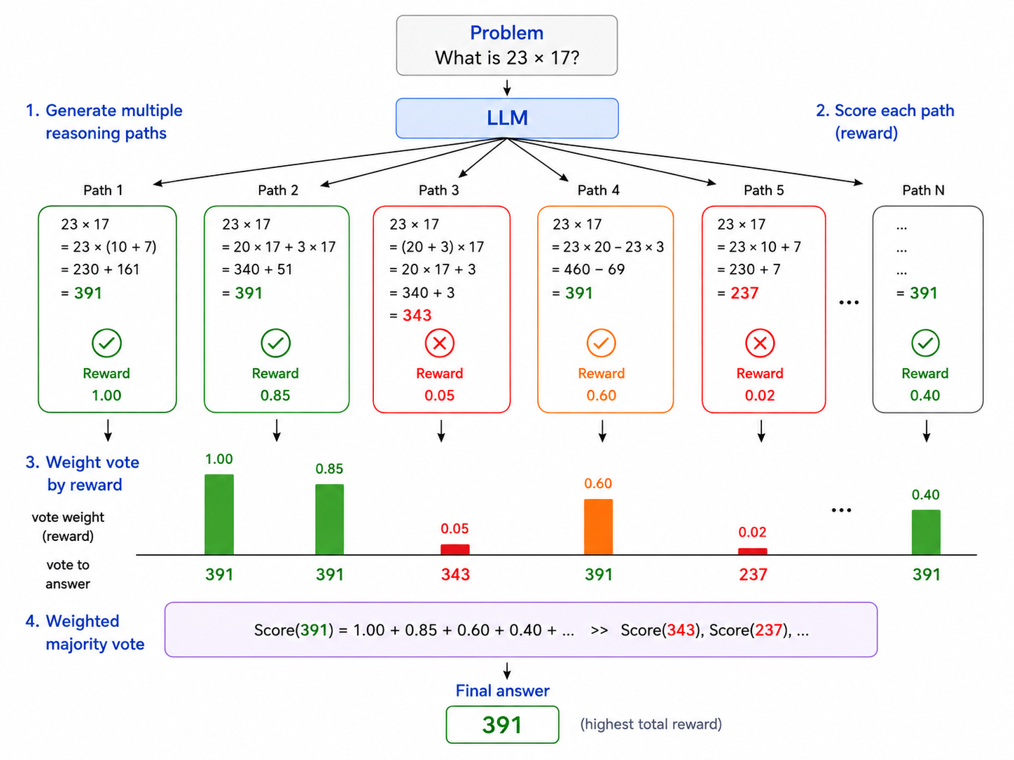
A related idea appears in reward-weighted majority voting for LLM reasoning: generate multiple candidate solutions, score them, and allow higher-scoring candidates to contribute more strongly to the final answer.
 \
\
If we use the base model itself as the proposal, $q(x)=p_{\mathrm{ref}}(x)$, the importance weight simplifies to
\[w(x) \propto \exp\left(-\frac{g(x)}{\beta}\right),\]which depends only on the objective value of the solution.
The Problem with Importance Sampling
Importance sampling has a fundamental weakness: when the proposal and target distributions are far apart, almost all samples receive negligible weight.
As a result, a huge number of samples may be required before we obtain meaningful coverage of the high-probability regions of the target distribution.
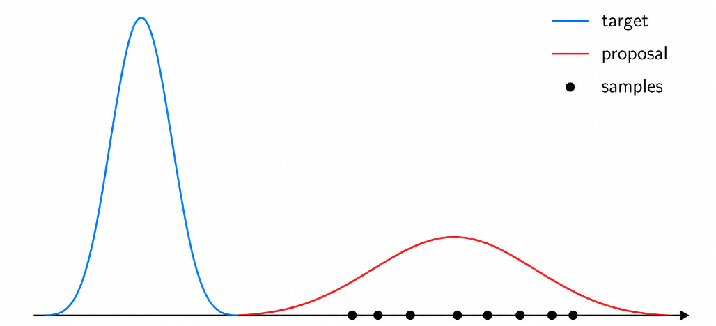
This problem becomes particularly severe for long reasoning trajectories. Even if the proposal differs only slightly from the target at each step, these discrepancies can accumulate over a long sequence, eventually making the two trajectory distributions very different.
A natural idea is therefore to correct the distribution along the way rather than waiting until the end.
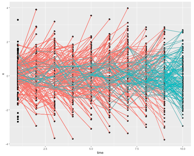
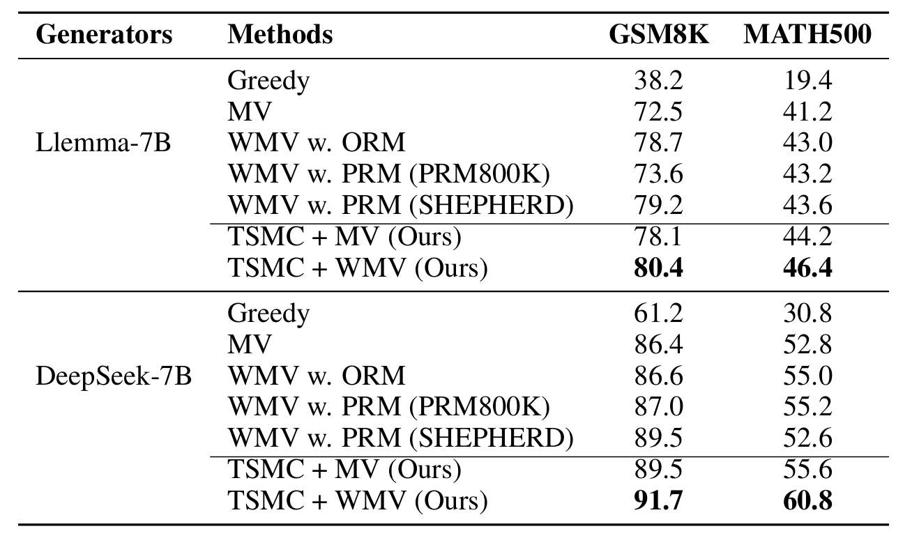
This leads us to Twisted Sequential Monte Carlo (TSMC), which I explored for LLM reasoning in my prior work.
3.2. Twisted Sequential Monte Carlo
Suppose a complete solution consists of $T$ steps,
\[x=(x_1,x_2,\ldots,x_T).\]Our target distribution over complete solutions is
\[p(x_{1:T}) \propto p_{\mathrm{ref}}(x_{1:T}) \exp\left(-\frac{g(x_{1:T})}{\beta}\right).\]But what should the target distribution look like after only $t$ steps?
We can obtain it by marginalizing over all possible future continuations:
\[p(x_{1:t}) \propto p_{\mathrm{ref}}(x_{1:t}) \underbrace{ \mathbb{E}_{x_{t+1:T}\sim p_{\mathrm{ref}}(\cdot\mid x_{1:t})} \left[ \exp\left(-\frac{g(x_{1:T})}{\beta}\right) \right] }_{V(x_{1:t})}.\]Here,
\[V(x_{1:t}) = \mathbb{E}_{x_{t+1:T}\sim p_{\mathrm{ref}}(\cdot\mid x_{1:t})} \left[ \exp\left(-\frac{g(x_{1:T})}{\beta}\right) \right]\]is a soft value function. It measures how promising a partial solution is by averaging over its possible future completions.
In practice, we can train a value network to approximate this quantity. Because the expectation is taken over continuations sampled from the base policy $p_{\mathrm{ref}}$, standard Monte Carlo regression is sufficient.
This reveals an important structure: the intermediate target has the same reward-tilted form as the final target, except that the final reward is replaced by the soft value $V(x_{1:t})$.
TSMC then follows naturally. Suppose that at step $t$ we have $n$ particles approximately distributed according to $p(x_{1:t})$.
-
Extend each particle using the base model:
\[x_{t+1}^i \sim p_{\mathrm{ref}}(\cdot\mid x_{1:t}^i).\] -
Reweight the resulting particles:
\[w^i \propto \frac{ V(x_{1:t+1}^i) }{ V(x_{1:t}^i) }.\] -
Resample $n$ particles according to their normalized weights.
Then repeat.
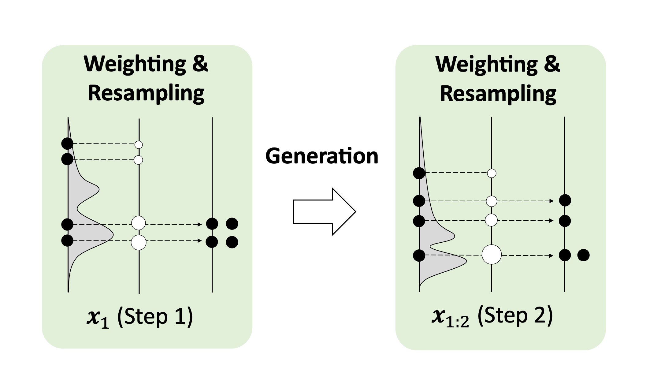
Importantly, TSMC maintains a fixed batch of $n$ sequences throughout sampling, with no variation in batch width, making the procedure naturally amenable to efficient parallelization, in contrast to Monte Carlo Tree Search (MCTS).
Instead of generating an entire solution and asking only at the end whether it was good, TSMC repeatedly asks:
Which partial solutions still have promising futures?
Unpromising trajectories can be discarded early, while promising ones receive more computation.
This highlights the key difference from importance sampling. Both methods can target the same distribution, but TSMC performs corrections throughout the trajectory rather than only after a complete solution has been generated. This can dramatically reduce variance for long-horizon problems such as mathematical reasoning.
3.3. Markov Chain Monte Carlo
Another classical approach for sampling from an EBM is Markov chain Monte Carlo (MCMC).
The core idea is simple. Instead of generating independent samples from scratch — which is hard when the target distribution is complex — MCMC constructs a chain of states that wanders through the space, spending more time in high-probability regions. Each state is obtained by randomly modifying the previous one, so the chain evolves gradually rather than making large random jumps.
Concretely, starting from a current state $x$, we propose a nearby state
\[x' \sim q(x'\mid x),\]and then decide whether to accept or reject the proposal. If the new state has higher probability than the current one, we always accept it. If it has lower probability, we accept it only with some chance — this randomness prevents the chain from getting stuck in a local mode. Over many steps, this accept/reject rule ensures the chain visits states in proportion to their probability under the target distribution.
The most classical version is Metropolis-Hastings, which accepts $x'$ with probability
\[A(x',x) = \min\left( 1, \frac{ p(x')q(x\mid x') }{ p(x)q(x'\mid x) } \right).\]A key convenience: the normalization constant cancels in the ratio, so we can run MCMC even when we only know $p(x)$ up to normalization — which is exactly our situation with the EBM.
Interestingly, this classical idea has recently reappeared in LLM reasoning. Karan & Du (2025) ask whether some of the benefits of RL post-training can instead be obtained purely through sampling.
Prior studies such as Yue et al. (2025) suggest a provocative interpretation of RL for reasoning: part of its benefit may come from reshaping the model's output distribution so that successful reasoning trajectories become much more likely under a single sample, rather than creating entirely new capabilities.
From this perspective, RL can be thought of as sharpening the distribution over reasoning trajectories.
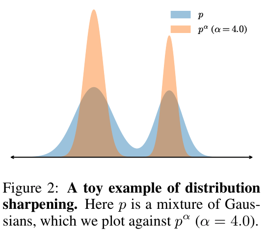
Motivated by this view, given a base model distribution $p_{\mathrm{ref}}(x)$, they consider a sharpened target distribution
\[p_\alpha(x) \propto p_{\mathrm{ref}}(x)^\alpha, \qquad \alpha>1,\]which places relatively more probability mass on sequences that the base model itself considers likely.
Importantly, this is not equivalent to simply lowering the token-level sampling temperature.
Standard temperature sampling locally sharpens each conditional distribution
\[p(x_t\mid x_{< t}),\]whereas the distribution above sharpens the probability of the entire sequence $p_{\mathrm{ref}}(x_{1:T})$.
We now have exactly the MCMC problem described above: $p_\alpha(x)$ is easy to evaluate (with the base model $p_{\mathrm{ref}}$) up to normalization but difficult to sample from directly.
The remaining question is therefore:
What should the proposal $q(x'\mid x)$ look like for a language model?
Their answer is particularly simple. Given a current sequence $x$, randomly pick a position in it, keep everything before that position unchanged (the prefix), and let the base language model freely regenerate everything from that position onward (the suffix):
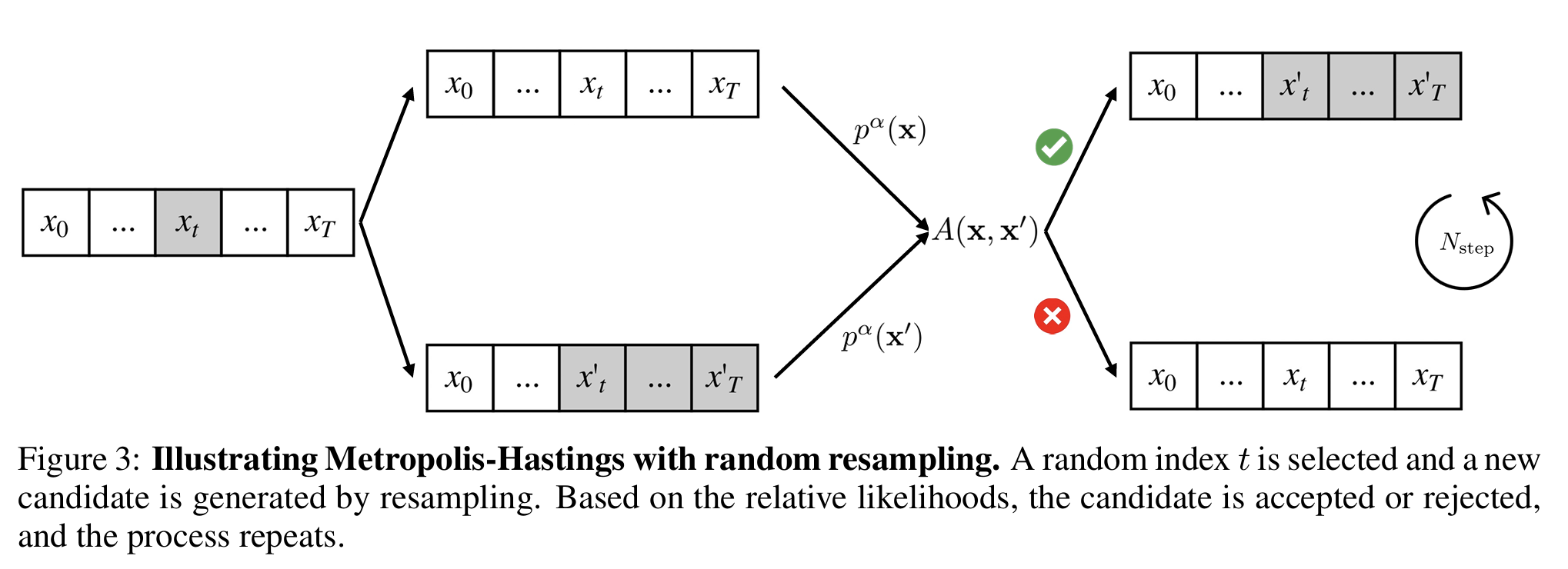
Formally, after sampling a random cut point $t \sim \text{Uniform}({1,\ldots,T})$, the proposal is:
\[q(x'\mid x) = p_{\mathrm{ref}}(x'_{t:T}\mid x_{1:t-1}), \quad \text{with } x'_{1:t-1} = x_{1:t-1}.\]In other words, the proposal is simply the base model conditioned on the shared prefix. This is easy to compute — it requires no extra training, just running the language model forward from the cut point.
Then apply the same Metropolis-Hastings accept/reject rule introduced above:
\[x' \quad\xrightarrow{\text{accept/reject}}\quad \begin{cases} x', & \text{accept},\\ x, & \text{reject}. \end{cases}\]The accepted sequence becomes the starting point for the next MCMC step. Repeating this process allows the model to continually revise its own reasoning trajectory, while the accept/reject step biases the samples toward the sharpened target distribution $p_{\mathrm{ref}}(x)^\alpha$.
There is still one difficulty: reasoning trajectories can be very long, making MCMC over the entire sequence difficult to mix.
Instead of immediately sampling a full trajectory, the authors therefore progressively increase the sequence length. Schematically,
\[\emptyset \rightarrow p(x_{0:B})^\alpha \rightarrow p(x_{0:2B})^\alpha \rightarrow \cdots \rightarrow p(x_{0:T})^\alpha.\]At each stage, they first extend the current sequence by another block of tokens and then perform several rounds of resample → accept/reject before moving to the next stage. The sample from one stage therefore provides a useful initialization for sampling the longer sequence at the next.
This practice is actually very similar to TSMC, except that they have multiple refinement at each step, turning SMC into Sequential MCMC.
The resulting procedure has a very different interpretation from RL. RL spends computation changing the model parameters so that desirable trajectories become more likely. Here, the model parameters never change. Instead, computation is spent iteratively revising and selecting samples from the base model itself.
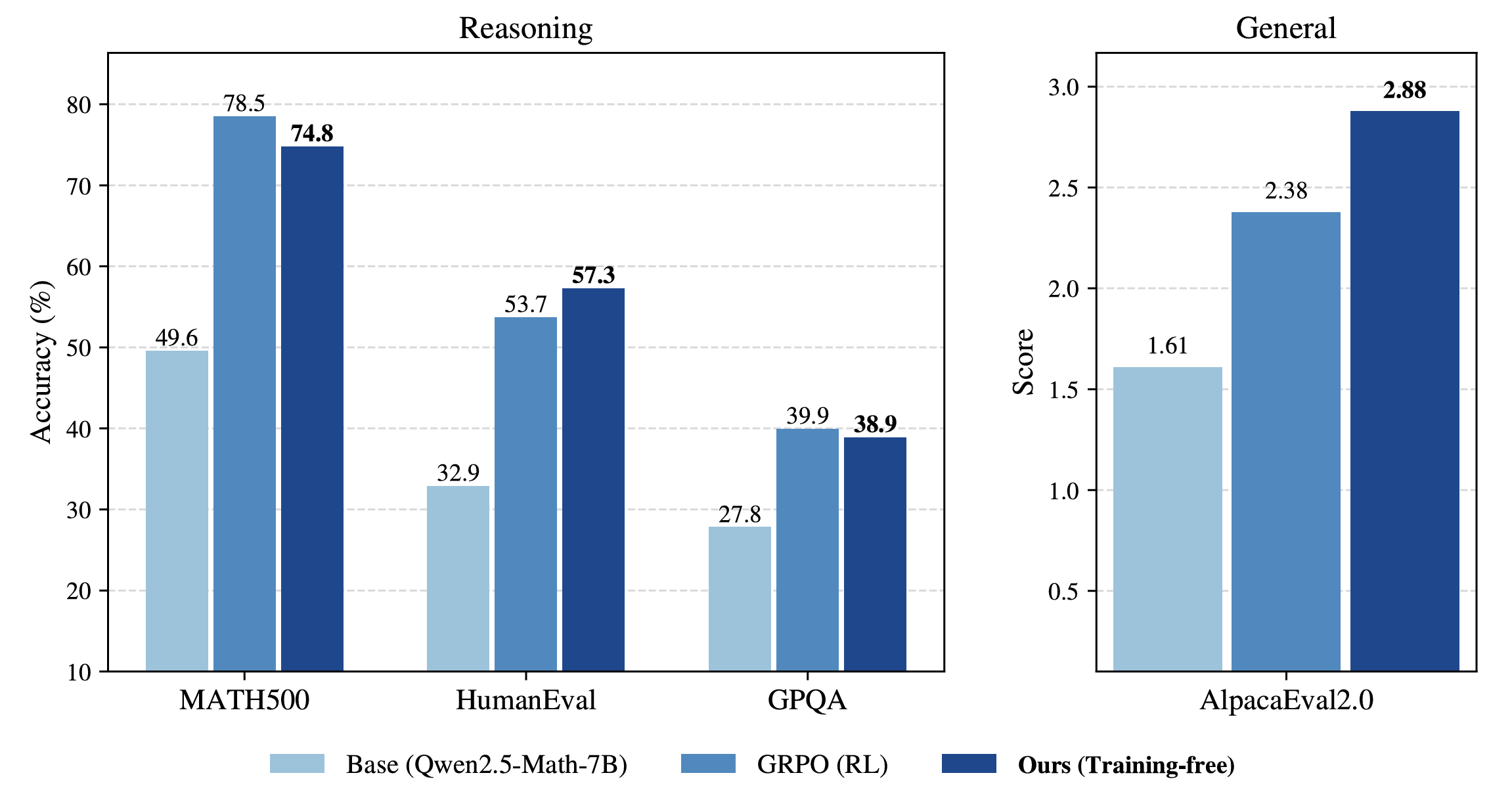
Remarkably, the paper shows that this training-free procedure can achieve reasoning performance comparable to RL post-training on several benchmarks.
Remark
At first glance, the sampling methods above may seem largely independent of neural network training. But in an RL-like setting, learning can often be viewed as two intertwined components: sampling and optimization.
If we can already obtain samples from, or sufficiently close to, a desired target distribution, the remaining problem can potentially be reduced to supervised learning: train the model to imitate these samples. This opens up a very different learning paradigm from directly optimizing the model with RL.
Importantly, this is also what distinguishes principled sampling methods from heuristic decoding strategies. Their outputs are not merely candidates that happen to score well; under appropriate assumptions, they can be justified as approximating a well-defined target distribution, making them potentially useful as supervised training signals.
How to tightly integrate advanced sampling methods with neural network training therefore remains an exciting direction to explore.